while my_mcmc: gently(samples) - The Inference Button: Bayesian GLMs made easy with PyMC

This post was updated in August 2026 to run on PyMC v6 (formerly PyMC3; using Bambi for the formula API).

This tutorial appeared as a post in a small series on Bayesian GLMs on my blog:

In this blog post I will talk about:

How the Bayesian Revolution in many scientific disciplines is hindered by poor usability of current Probabilistic Programming languages.
A gentle introduction to Bayesian linear regression and how it differs from the frequentist approach.
A preview of PyMC and its new GLM submodule I wrote to allow creation and estimation of Bayesian GLMs as easy as frequentist GLMs in R (this functionality lives on in Bambi, which this updated version of the post uses).

Ready? Lets get started!

There is a huge paradigm shift underway in many scientific disciplines: The Bayesian Revolution.

While the theoretical benefits of Bayesian over Frequentist stats have been discussed at length elsewhere (see Further Reading below), there is a major obstacle that hinders wider adoption – usability (this is one of the reasons DARPA wrote out a huge grant to improve Probabilistic Programming).

This is mildly ironic because the beauty of Bayesian statistics is their generality. Frequentist stats have a bazillion different tests for every different scenario. In Bayesian land you define your model exactly as you think is appropriate and hit the Inference Button(TM) (i.e. running the magical MCMC sampling algorithm).

Yet when I ask my colleagues why they use frequentist stats (even though they would like to use Bayesian stats) the answer is that software packages like SPSS or R make it very easy to run all those individuals tests with a single command (and more often then not, they don’t know the exact model and inference method being used).

While there are great Bayesian software packages like JAGS, BUGS, Stan and PyMC, they are written for Bayesians statisticians who know very well what model they want to build.

Unfortunately, “the vast majority of statistical analysis is not performed by statisticians” – so what we really need are tools for scientists and not for statisticians.

In the interest of putting my code where my mouth is I wrote a submodule for the upcoming PyMC that makes construction of Bayesian Generalized Linear Models (GLMs) as easy as Frequentist ones in R.

Linear Regression

While future blog posts will explore more complex models, I will start here with the simplest GLM – linear regression. In general, frequentists think about Linear Regression as follows:

\[ Y = X\beta + \epsilon \]

where \(Y\) is the output we want to predict (or dependent variable), \(X\) is our predictor (or independent variable), and \(\beta\) are the coefficients (or parameters) of the model we want to estimate. \(\epsilon\) is an error term which is assumed to be normally distributed.

We can then use Ordinary Least Squares or Maximum Likelihood to find the best fitting \(\beta\).

Probabilistic Reformulation

Bayesians take a probabilistic view of the world and express this model in terms of probability distributions. Our above linear regression can be rewritten to yield:

\[ Y \sim \mathcal{N}(X \beta, \sigma^2) \]

In words, we view \(Y\) as a random variable (or random vector) of which each element (data point) is distributed according to a Normal distribution. The mean of this normal distribution is provided by our linear predictor with variance \(\sigma^2\).

While this is essentially the same model, there are two critical advantages of Bayesian estimation:

Priors: We can quantify any prior knowledge we might have by placing priors on the paramters. For example, if we think that \(\sigma\) is likely to be small we would choose a prior with more probability mass on low values.
Quantifying uncertainty: We do not get a single estimate of \(\beta\) as above but instead a complete posterior distribution about how likely different values of \(\beta\) are. For example, with few data points our uncertainty in \(\beta\) will be very high and we’d be getting very wide posteriors.

Bayesian GLMs in PyMC

With Bambi, the successor to PyMC’s original GLM module, it is very easy to build this and much more complex models.

First, lets import the required modules.

%matplotlib inline

import arviz as az
import bambi as bmb
import matplotlib.pyplot as plt
import numpy as np
import pandas as pd
import pymc as pm

Generating data

Create some toy data to play around with and scatter-plot it.

Essentially we are creating a regression line defined by intercept and slope and add data points by sampling from a Normal with the mean set to the regression line.

size = 200
true_intercept = 1
true_slope = 2

x = np.linspace(0, 1, size)
# y = a + b*x
true_regression_line = true_intercept + true_slope * x
# add noise
y = true_regression_line + np.random.normal(scale=.5, size=size)

data = pd.DataFrame(dict(x=x, y=y))

fig = plt.figure(figsize=(7, 7))
ax = fig.add_subplot(111, xlabel='x', ylabel='y', title='Generated data and underlying model')
ax.plot(x, y, 'x', label='sampled data')
ax.plot(x, true_regression_line, label='true regression line', lw=2.)
plt.legend(loc=0);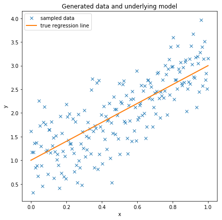

Estimating the model

Lets fit a Bayesian linear regression model to this data. As you can see, model specifications in PyMC are wrapped in a with statement.

Here we use the awesome new NUTS sampler (our Inference Button) to draw 2000 posterior samples.

with pm.Model() as model: # model specifications in PyMC are wrapped in a with-statement
    # Define priors
    sigma = pm.HalfCauchy('sigma', beta=10, initval=1.)
    intercept = pm.Normal('Intercept', 0, sigma=20)
    x_coeff = pm.Normal('x', 0, sigma=20)

    # Define likelihood
    likelihood = pm.Normal('y', mu=intercept + x_coeff * x,
                           sigma=sigma, observed=y)

    # Inference!
    trace = pm.sample(progressbar=False) # draw posterior samples using NUTS sampling

This should be fairly readable for people who know probabilistic programming. However, would my non-statistican friend know what all this does? Moreover, recall that this is an extremely simple model that would be one line in R. Having multiple, potentially transformed regressors, interaction terms or link-functions would also make this much more complex and error prone.

Bambi, the successor to PyMC’s original glm() function, instead takes an R-style linear model specifier from which it creates a design matrix. bmb.Model() then adds random variables for each of the coefficients and an appropriate likelihood to the model.

# specify the model and pass in data. The resulting linear model, its likelihood and
# all its parameters are automatically added to our model.
model = bmb.Model('y ~ x', data)
trace = model.fit(tune=1000, cores=4, progressbar=False) # draw posterior samples using NUTS sampling

Much shorter, but this code does the exact same thing as the above model specification (you can change priors and everything else too if we wanted). bmb.Model() parses the model string, adds random variables for each regressor (Intercept and slope x in this case), adds a likelihood (by default, a Normal is chosen), and all other variables (sigma). Finally, Bambi assigns sensible default priors informed by the data.

If you are not familiar with R’s syntax, 'y ~ x' specifies that we have an output variable y that we want to estimate as a linear function of x.

Analyzing the model

Bayesian inference does not give us only one best fitting line (as maximum likelihood does) but rather a whole posterior distribution of likely parameters. Lets plot the posterior distribution of our parameters and the individual samples we drew.

az.plot_trace_dist(trace);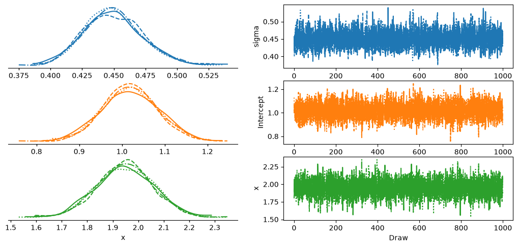

The left side shows our marginal posterior – for each parameter value on the x-axis we get a probability on the y-axis that tells us how likely that parameter value is.

There are a couple of things to see here. The first is that our sampling chains for the individual parameters (left side) seem well converged and stationary (there are no large drifts or other odd patterns). We see 4 lines because we ran 4 chains in parallel (cores parameter above). They all seem to provide the same answer which is re-assuring.

Secondly, the maximum posterior estimate of each variable (the peak in the left side distributions) is very close to the true parameters used to generate the data (x is the regression coefficient and sigma is the standard deviation of our normal).

In the GLM we thus do not only have one best fitting regression line, but many. A posterior predictive plot takes multiple samples from the posterior (intercepts and slopes) and plots a regression line for each of them. Here we draw 100 samples of intercept and slope from the posterior and plot the corresponding regression lines.

plt.figure(figsize=(7, 7))
plt.plot(x, y, 'x', label='data')

# plot posterior predictive regression lines from 100 posterior samples
post = az.extract(trace, num_samples=100)
lines = post['Intercept'].values + post['x'].values * x[:, None]
plt.plot(x, lines, c='C1', alpha=.1)
plt.plot([], [], c='C1', label='posterior predictive regression lines')

plt.plot(x, true_regression_line, label='true regression line', lw=3., c='y')

plt.title('Posterior predictive regression lines')
plt.legend(loc=0)
plt.xlabel('x')
plt.ylabel('y');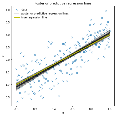

As you can see, our estimated regression lines are very similar to the true regression line. But since we only have limited data we have uncertainty in our estimates, here expressed by the variability of the lines.

Summary

Usability is currently a huge hurdle for wider adoption of Bayesian statistics.
PyMC (via Bambi) allows GLM specification with convenient syntax borrowed from R.
Posterior predictive plots allow us to evaluate fit and our uncertainty in it.