while my_mcmc: gently(samples) - Random-Walk Bayesian Deep Networks: Dealing with Non-Stationary Data

This post was updated in August 2026 to run on PyMC v6 (formerly PyMC3; PyTensor backend).

Most problems solved by Deep Learning are stationary. A cat is always a cat. The rules of Go have remained stable for 2,500 years, and will likely stay that way. However, what if the world around you is changing? This is common, for example when applying Machine Learning in Quantitative Finance. Markets are constantly evolving so features that are predictive in some time-period might lose their edge, while other patterns emerge. Usually, quants would just retrain their classifiers every once in a while. This approach of just re-estimating the same model on more recent data is very common. I find that to be a pretty unsatisfying way of modeling, as there are certain shortfalls:

The estimation window should be long so as to incorporate as much training data as possible.
The estimation window should be short so as to incorporate only the most recent data, as old data might be obsolete.
When you have no estimate of how fast the world around you is changing, there is no principled way of setting the window length to balance these two objectives.

Certainly there is something to be learned even from past data, we just need to instill our models with a sense of time and recency.

Enter random-walk processes. Ever since I learned about them in the stochastic volatility model they have become one of my favorite modeling tricks. Basically, it allows you to turn every static model into a time-sensitive one.

You can read more about the details of a random-walk priors here, but the central idea is that, in any time-series model, rather than assuming a parameter to be constant over time, we allow it to change gradually, following a random walk. For example, take a logistic regression:

\[ Y_i = f(\beta X_i) \]

Where \(f\) is the logistic function and \(\beta\) is our learnable parameter. If we assume that our data is not iid and that \(\beta\) is changing over time. We thus need a different \(\beta\) for every \(i\):

\[ Y_i = f(\beta_i X_i) \]

Of course, this will just overfit, so we need to constrain our \(\beta_i\) somehow. We will assume that while \(\beta_i\) is changing over time, it will do so rather gradually by placing a random-walk prior on it:

\[ \beta_t \sim \mathcal{N}(\beta_{t-1}, s^2) \]

So \(\beta_t\) is allowed to only deviate a little bit (determined by the step-width \(s\)) form its previous value \(\beta_{t-1}\). \(s\) can be thought of as a stability parameter – how fast is the world around you changing.

Let’s first generate some toy data and then implement this model in PyMC. We will then use this same trick in a Neural Network with hidden layers.

If you would like a more complete introduction to Bayesian Deep Learning, see my recent ODSC London talk. This blog post takes things one step further so definitely read further below.

%matplotlib inline
import pymc as pm
import pytensor
import pytensor.tensor as pt
import arviz as az
import sklearn
import numpy as np
import matplotlib.pyplot as plt
import seaborn as sns
sns.set_style('white')
from sklearn import datasets
from sklearn.preprocessing import scale

sns.set_context('notebook')

Generating data

First, lets generate some toy data – a simple binary classification problem that’s linearly separable. To introduce the non-stationarity, we will rotate this data along the center across time. Safely skip over the next few code cells.

X, Y = sklearn.datasets.make_blobs(n_samples=1000, centers=2, random_state=1)
X = scale(X)
colors = Y.astype(str)
colors[Y == 0] = 'r'
colors[Y == 1] = 'b'

interval = 20
subsample = X.shape[0] // interval
chunk = np.arange(0, X.shape[0]+1, subsample)
degs = np.linspace(0, 360, len(chunk))

sep_lines = []

for ii, (i, j, deg) in enumerate(list(zip(np.roll(chunk, 1), chunk, degs))[1:]):
    theta = np.radians(deg)
    c, s = np.cos(theta), np.sin(theta)
    R = np.matrix([[c, -s], [s, c]])

    X[i:j, :] = X[i:j, :].dot(R)

import base64

VIDEO_TAG = """<video controls>
 <source src="data:video/x-m4v;base64,{0}" type="video/mp4">
 Your browser does not support the video tag.
</video>"""


def anim_to_html(anim):
    if not hasattr(anim, '_encoded_video'):
        anim.save("test.mp4", fps=20, extra_args=['-vcodec', 'libx264'])

        video = open("test.mp4","rb").read()

        anim._encoded_video = base64.b64encode(video).decode('utf-8')
    return VIDEO_TAG.format(anim._encoded_video)

from IPython.display import HTML

def display_animation(anim):
    plt.close(anim._fig)
    return HTML(anim_to_html(anim))
from matplotlib import animation

# First set up the figure, the axis, and the plot element we want to animate
fig, ax = plt.subplots()
ims = [] #l, = plt.plot([], [], 'r-')
for i in np.arange(0, len(X), 10):
    ims.append([(ax.scatter(X[:i, 0], X[:i, 1], color=colors[:i]))])

ax.set(xlabel='X1', ylabel='X2')
# call the animator.  blit=True means only re-draw the parts that have changed.
anim = animation.ArtistAnimation(fig, ims,
                                 interval=500,
                                 blit=True);

display_animation(anim)

The last frame of the video, where all data is plotted is what a classifier would see that has no sense of time. Thus, the problem we set up is impossible to solve when ignoring time, but trivial once you do.

How would we classically solve this? You could just train a different classifier on each subset. But as I wrote above, you need to get the frequency right and you use less data overall.

Random-Walk Logistic Regression in PyMC

n_dim = X.shape[1] # 2

with pm.Model() as random_walk_perceptron:
    X_data = pm.Data('X_data', X)
    Y_data = pm.Data('Y_data', Y)

    step_size = pm.HalfNormal('step_size', sigma=np.ones(n_dim),
                              shape=n_dim)

    # This is the central trick, PyMC already comes with this distribution.
    # Since PyMC v4 the random walk evolves along the *last* axis, so we
    # parametrize the weights as (n_dim, interval) and transpose below.
    w = pm.GaussianRandomWalk('w', sigma=step_size,
                              init_dist=pm.Normal.dist(0, 10),
                              shape=(n_dim, interval))

    weights = pt.repeat(w.T, X_data.shape[0] // interval, axis=0)

    class_prob = pm.math.sigmoid((X_data * weights).sum(axis=-1))

    # Binary classification -> Bernoulli likelihood
    pm.Bernoulli('out', class_prob, observed=Y_data)

OK, if you understand the stochastic volatility model, the first two lines should look fairly familiar. We are creating 2 random-walk processes. As allowing the weights to change on every new data point is overkill, we subsample. The repeat turns the vector [t, t+1, t+2] into [t, t, t, t+1, t+1, ...] so that it matches the number of data points.

Next, we would usually just apply a single dot-product but here every data point comes with its own weight vector, so we take the row-wise product of the data with its weights and sum – the same thing a batched dot-product would do. In the end, we just get probabilities (predicitions) for our Bernoulli likelihood.

On to the inference. PyMC automatically initializes NUTS with a good starting point and mass matrix, so just calling pm.sample() usually runs quite robustly.

with random_walk_perceptron:
    trace_perceptron = pm.sample(2000, chains=2, cores=1, random_seed=42)

Let’s look at the learned weights over time:

w_post = az.extract(trace_perceptron, var_names='w', num_samples=500, random_seed=42)
plt.plot(w_post[0].values, alpha=.05, color='r');
plt.plot(w_post[1].values, alpha=.05, color='b');
plt.xlabel('time'); plt.ylabel('weights'); plt.title('Optimal weights change over time'); sns.despine();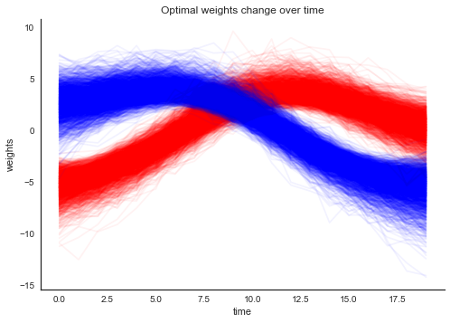

As you can see, the weights are slowly changing over time. What does the learned hyperplane look like? In the plot below, the points are still the training data but the background color codes the class probability learned by the model.

grid = np.mgrid[-3:3:100j,-3:3:100j]
grid_2d = grid.reshape(2, -1).T
grid_2d = np.tile(grid_2d, (interval, 1))
dummy_out = np.ones(grid_2d.shape[0], dtype=np.int8)

# Create posterior predictive samples on a thinned trace (~250 samples)
with random_walk_perceptron:
    pm.set_data({'X_data': grid_2d, 'Y_data': dummy_out})
    n_samples = trace_perceptron.posterior.sizes['chain'] * trace_perceptron.posterior.sizes['draw']
    thinned_trace = trace_perceptron.sel(draw=slice(None, None, max(1, n_samples // 250)))
    ppc = pm.sample_posterior_predictive(thinned_trace, random_seed=42)

ppc_out = ppc.posterior_predictive['out'].mean(('chain', 'draw')).values

def create_surface(X, Y, grid, ppc_vals, fig=None, ax=None):
    artists = []
    cmap = sns.diverging_palette(250, 12, s=85, l=25, as_cmap=True)
    contour = ax.contourf(*grid, ppc_vals, cmap=cmap)
    artists.append(contour)
    artists.append(ax.scatter(X[Y==0, 0], X[Y==0, 1], color='b'))
    artists.append(ax.scatter(X[Y==1, 0], X[Y==1, 1], color='r'))
    _ = ax.set(xlim=(-3, 3), ylim=(-3, 3), xlabel='X1', ylabel='X2');
    return artists

fig, ax = plt.subplots()
chunk = np.arange(0, X.shape[0]+1, subsample)
chunk_grid = np.arange(0, grid_2d.shape[0]+1, 10000)
axs = []
for (i, j), (i_grid, j_grid) in zip((list(zip(np.roll(chunk, 1), chunk))[1:]), (list(zip(np.roll(chunk_grid, 1), chunk_grid))[1:])):
    a = create_surface(X[i:j], Y[i:j], grid, ppc_out[i_grid:j_grid].reshape(100, 100), fig=fig, ax=ax)
    axs.append(a)

anim2 = animation.ArtistAnimation(fig, axs,
                                 interval=1000);
display_animation(anim2)

Nice, we can see that the random-walk logistic regression adapts its weights to perfectly separate the two point clouds.

Random-Walk Neural Network

In the previous example, we had a very simple linearly classifiable problem. Can we extend this same idea to non-linear problems and build a Bayesian Neural Network with weights adapting over time?

If you haven’t, I recommend you read my original post on Bayesian Deep Learning where I more thoroughly explain how a Neural Network can be implemented and fit in PyMC.

Lets generate some toy data that is not linearly separable and again rotate it around its center.

from sklearn.datasets import make_moons
X, Y = make_moons(noise=0.2, random_state=0, n_samples=5000)
X = scale(X)

colors = Y.astype(str)
colors[Y == 0] = 'r'
colors[Y == 1] = 'b'

interval = 20
subsample = X.shape[0] // interval
chunk = np.arange(0, X.shape[0]+1, subsample)
degs = np.linspace(0, 360, len(chunk))

sep_lines = []

for ii, (i, j, deg) in enumerate(list(zip(np.roll(chunk, 1), chunk, degs))[1:]):
    theta = np.radians(deg)
    c, s = np.cos(theta), np.sin(theta)
    R = np.matrix([[c, -s], [s, c]])

    X[i:j, :] = X[i:j, :].dot(R)

fig, ax = plt.subplots()
ims = []
for i in np.arange(0, len(X), 10):
    ims.append((ax.scatter(X[:i, 0], X[:i, 1], color=colors[:i]),))

ax.set(xlabel='X1', ylabel='X2')
anim = animation.ArtistAnimation(fig, ims,
                                 interval=500, 
                                 blit=True);

display_animation(anim)

Looks a bit like Ying and Yang, who knew we’d be creating art in the process.

On to the model. Rather than have all the weights in the network follow random-walks, we will just have the first hidden layer change its weights. The idea is that the higher layers learn stable higher-order representations while the first layer is transforming the raw data so that it appears stationary to the higher layers. We can of course also place random-walk priors on all weights, or only on those of higher layers, whatever assumptions you want to build into the model.

np.random.seed(123)

n_hidden = [2, 5]

# Initialize random weights between each layer
init_1 = np.random.randn(X.shape[1], n_hidden[0]).astype(pytensor.config.floatX)
init_2 = np.random.randn(n_hidden[0], n_hidden[1]).astype(pytensor.config.floatX)
init_out = np.random.randn(n_hidden[1]).astype(pytensor.config.floatX)

with pm.Model() as neural_network:
    ann_input = pm.Data('ann_input', X)
    ann_output = pm.Data('ann_output', Y)

    # Weights from input to hidden layer: one random-walk process per weight.
    # We build the Gaussian random walk in its non-centered form --
    # standard-normal innovations scaled by the step-size, then cumulatively
    # summed -- which gives NUTS a much easier geometry to sample.
    # Time is the last axis: (n_in, n_hidden, interval).
    step_size = pm.HalfNormal('step_size', sigma=np.ones(n_hidden[0]),
                              shape=n_hidden[0])

    w1_innov = pm.Normal('w1_innov', mu=0, sigma=1.,
                         shape=(X.shape[1], n_hidden[0], interval),
                         initval=np.concatenate([init_1[:, :, None],
                                                 np.zeros((X.shape[1], n_hidden[0], interval - 1))],
                                                axis=-1))
    innovations = pt.concatenate([w1_innov[..., :1],
                                  w1_innov[..., 1:] * step_size[None, :, None]],
                                 axis=-1)
    weights_in_1 = pm.Deterministic('w1', pt.cumsum(innovations, axis=-1))

    # Weights of the higher layers are stable across time
    weights_1_2 = pm.Normal('w2', mu=0, sigma=1.,
                            shape=(n_hidden[0], n_hidden[1]),
                            initval=init_2)

    weights_2_out = pm.Normal('w3', mu=0, sigma=1.,
                              shape=(n_hidden[1],),
                              initval=init_out)

    # Reshape the data into (interval, n_data_per_interval, n_in) blocks so
    # that each time-interval is matrix-multiplied with its own set of
    # first-layer weights
    ann_input_t = ann_input.reshape((interval, -1, X.shape[1]))
    weights_in_1_t = pt.moveaxis(weights_in_1, -1, 0)  # -> (interval, n_in, n_hidden)

    # Build neural-network using tanh activation function
    act_1 = pt.tanh(pt.matmul(ann_input_t,
                              weights_in_1_t))
    act_2 = pt.tanh(pt.dot(act_1,
                           weights_1_2))
    act_out = pm.math.sigmoid(pt.dot(act_2,
                                     weights_2_out))

    # Binary classification -> Bernoulli likelihood
    out = pm.Bernoulli('out',
                       act_out,
                       observed=ann_output.reshape((interval, -1)))

Hopefully that’s not too incomprehensible. It is basically applying the principles from the random-walk logistic regression but adding another hidden layer. One difference: rather than using the GaussianRandomWalk distribution directly, here we construct the random walk manually in its non-centered form, which samples much more efficiently in this deeper model.

I also want to take the opportunity to look at what the Bayesian approach to Deep Learning offers. Usually, we fit these models using point-estimates like the MLE or the MAP. Let’s see how well that works on a structually more complex model like this one:

with neural_network:
    map_est = pm.find_MAP()

plt.plot(map_est['w1'].reshape(-1, interval).T);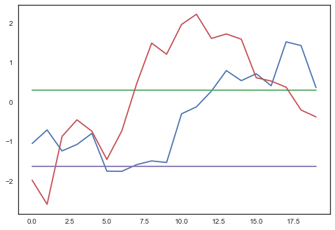

Some of the weights are changing, maybe it worked? How well does it fit the training data:

ppc = pm.sample_posterior_predictive([map_est], model=neural_network, random_seed=42)
print('Accuracy on train data = {:.2f}%'.format((ppc.posterior_predictive['out'].values[0, 0].ravel() == Y).mean() * 100))

Accuracy on train data = 95.80%

Now on to estimating the full posterior, as a proper Bayesian would:

with neural_network:
    trace = pm.sample(1000, tune=500, chains=2, cores=1,
                      init='advi+adapt_diag', n_init=30_000,
                      random_seed=42)

Finished [100%]: Average Loss = 1,354.7
There was 1 divergence after tuning. Increase `target_accept` or reparameterize.

w1_post = az.extract(trace, var_names='w1', num_samples=500, random_seed=42)
plt.plot(w1_post[0, 0].values, alpha=.05, color='r');
plt.plot(w1_post[0, 1].values, alpha=.05, color='b');
plt.plot(w1_post[1, 0].values, alpha=.05, color='g');
plt.plot(w1_post[1, 1].values, alpha=.05, color='c');

plt.xlabel('time'); plt.ylabel('weights'); plt.title('Optimal weights change over time'); sns.despine();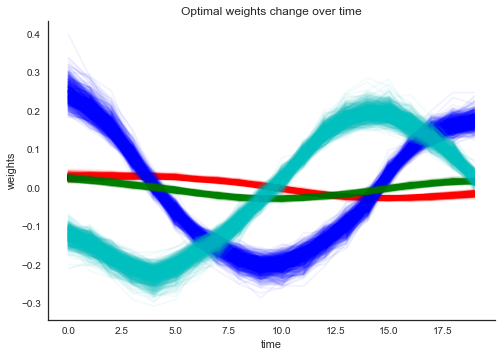

That already looks quite different. What about the accuracy:

n_samples = trace.posterior.sizes['chain'] * trace.posterior.sizes['draw']
thinned_trace = trace.sel(draw=slice(None, None, max(1, n_samples // 100)))
ppc = pm.sample_posterior_predictive(thinned_trace, model=neural_network, random_seed=42)
out_mean = ppc.posterior_predictive['out'].mean(('chain', 'draw')).values.ravel()
print('Accuracy on train data = {:.2f}%'.format(((out_mean > .5) == Y).mean() * 100))

Accuracy on train data = 96.96%

I think this is worth highlighting. In the original version of this post, the point-estimate did not do well at all – it barely beat chance – while estimating the whole posterior modeled the data much more accurately. Interestingly, with today’s PyMC (and the non-centered parametrization of the random walk above) the optimizer actually finds a decent mode, so the gap in raw accuracy has narrowed. The full posterior still fits better, and unlike the point-estimate it also quantifies its own uncertainty, as we will see below. In general the MAP remains a risky choice in models like this: the optimizer can get stuck because it can’t deal with the correlations in the posterior as well as NUTS can, and the MAP may just not be a good point. See my other blog post on hierarchical models as for why the MAP is a terrible choice for some models.

On to the fireworks. What does this actually look like:

grid = np.mgrid[-3:3:100j,-3:3:100j]
grid_2d = grid.reshape(2, -1).T
grid_2d = np.tile(grid_2d, (interval, 1))
dummy_out = np.ones(grid_2d.shape[0], dtype=np.int8)

# Create posterior predictive samples on a thinned trace (~250 samples)
with neural_network:
    pm.set_data({'ann_input': grid_2d, 'ann_output': dummy_out})
    thinned_trace = trace.sel(draw=slice(None, None, max(1, n_samples // 250)))
    ppc = pm.sample_posterior_predictive(thinned_trace, random_seed=42)

ppc_mean = ppc.posterior_predictive['out'].mean(('chain', 'draw')).values.ravel()

fig, ax = plt.subplots()
chunk = np.arange(0, X.shape[0]+1, subsample)
chunk_grid = np.arange(0, grid_2d.shape[0]+1, 10000)
axs = []
for (i, j), (i_grid, j_grid) in zip((list(zip(np.roll(chunk, 1), chunk))[1:]), (list(zip(np.roll(chunk_grid, 1), chunk_grid))[1:])):
    a = create_surface(X[i:j], Y[i:j], grid, ppc_mean[i_grid:j_grid].reshape(100, 100), fig=fig, ax=ax)
    axs.append(a)

anim2 = animation.ArtistAnimation(fig, axs,
                                  interval=1000);
display_animation(anim2)

Holy shit! I can’t believe that actually worked. Just for fun, let’s also make use of the fact that we have the full posterior and plot our uncertainty of our prediction (the background now encodes posterior standard-deviation where red means high uncertainty).

ppc_std = ppc.posterior_predictive['out'].std(('chain', 'draw')).values.ravel()

fig, ax = plt.subplots()
chunk = np.arange(0, X.shape[0]+1, subsample)
chunk_grid = np.arange(0, grid_2d.shape[0]+1, 10000)
axs = []
for (i, j), (i_grid, j_grid) in zip((list(zip(np.roll(chunk, 1), chunk))[1:]), (list(zip(np.roll(chunk_grid, 1), chunk_grid))[1:])):
    a = create_surface(X[i:j], Y[i:j], grid, ppc_std[i_grid:j_grid].reshape(100, 100),
                       fig=fig, ax=ax)
    axs.append(a)

anim2 = animation.ArtistAnimation(fig, axs,
                                  interval=1000);
display_animation(anim2)

Conclusions

In this blog post I explored the possibility of extending Neural Networks in new ways (to my knowledge), enabled by expressing them in a Probabilistic Programming framework. Full posterior inference using MCMC fit this model well and – unlike a classic point-estimate, which failed badly in the original version of this post – also provides us with the uncertainty of the predictions. What is quite nice, is that we did not have to do anything special for the inference in PyMC, just calling pymc.sample() gave stable results on this complex model.

Initially I built the model allowing all parameters to change, but realizing that we can selectively choose which layers to change felt like a profound insight. If you expect the raw data to change, but the higher-level representations to remain stable, as was the case here, we allow the bottom hidden layers to change. If we instead imagine e.g. handwriting recognition, where your handwriting might change over time, we would expect lower level features (lines, curves) to remain stable but allow changes in how we combine them. Finally, if the world remains stable but the labels change, we would place a random-walk process on the output layer. Of course, if you don’t know, you can have every layer change its weights over time and give each one a separate step-size parameter which would allow the model to figure out which layers change (high step-size), and which remain stable (low step-size).

In terms of quantatitative finance, this type of model allows us to train on much larger data sets ranging back a long time. A lot of that data is still useful to build up stable hidden representations, even if for predicition you still want your model to predict using its most up-to-date state of the world. No need to define a window-length or discard valuable training data.

%load_ext watermark
%watermark -v -m -p numpy,scipy,sklearn,pytensor,pymc,arviz,matplotlib

Python implementation: CPython
Python version       : 3.12.10
IPython version      : 9.17.0

numpy     : 2.4.6
scipy     : 1.18.1
sklearn   : 1.9.0
pytensor  : 3.3.0
pymc      : 6.3.1
arviz     : 1.3.0
matplotlib: 3.11.1

Compiler    : Clang 17.0.0 (clang-1700.0.13.3)
OS          : Darwin
Release     : 25.5.0
Machine     : arm64
Processor   : arm
CPU cores   : 8
Architecture: 64bit