%matplotlib inline
import numpy as np
from scipy import stats
import matplotlib.pyplot as plt
import seaborn as sns
from warnings import filterwarnings

import pymc3 as pm
from pymc3 import floatX
import theano
import theano.tensor as tt
from pymc3.theanof import set_tt_rng, MRG_RandomStreams

import sklearn
from sklearn import datasets
from sklearn.preprocessing import scale
from sklearn.model_selection import train_test_split
from sklearn.datasets import make_moons

filterwarnings('ignore')
sns.set_style('white')

set_tt_rng(MRG_RandomStreams(42))

cmap = sns.diverging_palette(250, 12, s=85, l=25, as_cmap=True)
cmap_uncertainty = sns.cubehelix_palette(light=1, as_cmap=True)

layer_names = ['w_in_1_grp', 'w_1_2_grp', 'w_2_out_grp']Imagine you have a machine learning (ML) problem but only small data (gasp, yes, this does exist). This often happens when your data set is nested – you might have many data points, but only few per category. For example, in ad-tech you may want predict how likely a user will buy a certain product. There could be thousands of products but you only have a small number of measurements (e.g. purchase decisions) per item. Likely, there will be similarities between each product category, but they will all have individual differences too.
Using classic ML methods is unlikely to yield good results in this setting. Firstly, ML is happiest with lots of data. If you want to be fancy and use deep learning, that usually requires even more data to give good performance. Moreover, we can’t really make use of the hierarchical structure (product-groupings) we know to be present in our data. So we can then either ignore it and try to learn one model for all categories which does not allow us to capture the differences between categories; or we can fit a ML model to each category separately but do not exploit the similarities between categories. (Technically, you could add the category as a feature and fit a single model but when I tried it on the data presented futher below it was at chance).
Hierarchical Bayesian models work amazingly well in exactly this setting as they allow us to build a model that matches the hierarchical structure present in our data set. Check out my previous blog post The Best Of Both Worlds: Hierarchical Linear Regression in PyMC3 for a refresher.
In this setting we could likely build a hierarchical logistic Bayesian model using PyMC3. However, what if our decision surface is actually more complex and a linear model would not give good performance?
In this blog post I explore how we can take a Bayesian Neural Network (BNN) and turn it into a hierarchical one. Once we built this model we derive an informed prior from it that we can apply back to a simple, non-hierarchical BNN to get the same performance as the hierachical one.
In the ML community, this problem is referred to as multitask transfer learning. Neural networks trained to play multiple Atari games have a hard time because they tend to forget what they learned before fairly quickly when trained on subsequent tasks (catastrophic forgetting), as the old weights get overwritten. Hierarchical BNNs can provide an elegant solution to this problem by sharing the higher-order representations that are useful but still allowing every subnetwork to specialize in a single task.
The data set we are using are our battle tested half-moons as it is simple, non-linear and leads to pretty visualizations. This is what it looks like:
X, Y = make_moons(noise=0.3, n_samples=1000)
plt.scatter(X[Y==0, 0], X[Y==0, 1], label='Class 0')
plt.scatter(X[Y==1, 0], X[Y==1, 1], color='r', label='Class 1')
sns.despine(); plt.legend();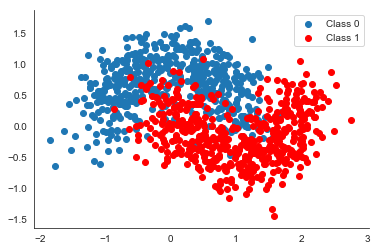
This is just to illustrate what the data generating distribution looks like, we will use way fewer data points, and create different subsets with different rotations.
def rotate(X, deg):
    theta = np.radians(deg)
    c, s = np.cos(theta), np.sin(theta)
    R = np.matrix([[c, -s], [s, c]])

    X = X.dot(R)

return np.asarray(X)np.random.seed(31)
n_samples = 100
n_grps = 18
n_grps_sq = int(np.sqrt(n_grps))
Xs, Ys = [], []
for i in range(n_grps):
# Generate data with 2 classes that are not linearly separable
X, Y = make_moons(noise=0.3, n_samples=n_samples)
X = scale(X)
X = floatX(X)
Y = floatX(Y)
# Rotate the points randomly for each category
rotate_by = np.random.randn() * 90.
X = rotate(X, rotate_by)
Xs.append(X)
Ys.append(Y)
Xs = np.stack(Xs)
Ys = np.stack(Ys)
Xs_train = Xs[:, :n_samples // 2, :]
Xs_test = Xs[:, n_samples // 2:, :]
Ys_train = Ys[:, :n_samples // 2]
Ys_test = Ys[:, n_samples // 2:]fig, axs = plt.subplots(figsize=(15, 12), nrows=n_grps_sq, ncols=n_grps_sq,
sharex=True, sharey=True)
axs = axs.flatten()
for i, (X, Y, ax) in enumerate(zip(Xs_train, Ys_train, axs)):
ax.scatter(X[Y==0, 0], X[Y==0, 1], label='Class 0')
ax.scatter(X[Y==1, 0], X[Y==1, 1], color='r', label='Class 1')
sns.despine(); ax.legend()
ax.set(title='Category {}'.format(i + 1), xlabel='X1', ylabel='X2')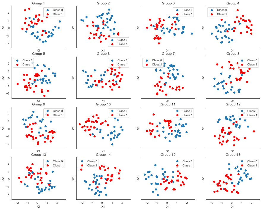
As you can see, we have 18 categories that share a higher-order structure (the half-moons). However, in the pure data space, no single classifier will be able to do a good job here. Also, because we only have 50 data points in each class, a NN will likely have a hard time producing robust results. But let’s actually test this.
Classify each category separately
The code for the NN below is explained in my previous blog post on Bayesian Deep Learning.
def construct_flat_nn(ann_input, ann_output):
    """Function to create a flat BNN given data."""
    n_hidden = 5

    # Initialize random weights between each layer
    init_1 = floatX(np.random.randn(X.shape[1], n_hidden))
    init_2 = floatX(np.random.randn(n_hidden, n_hidden))
    init_out = floatX(np.random.randn(n_hidden))

    with pm.Model() as neural_network:
        # Weights from input to hidden layer
        weights_in_1 = pm.Normal('w_in_1', 0, sd=1,
                                 shape=(X.shape[1], n_hidden),
                                 testval=init_1)

        # Weights from 1st to 2nd layer
        weights_1_2 = pm.Normal('w_1_2', 0, sd=1,
                                shape=(n_hidden, n_hidden),
                                testval=init_2)

        # Weights from hidden layer to output
        weights_2_out = pm.Normal('w_2_out', 0, sd=1,
                                  shape=(n_hidden,),
                                  testval=init_out)

        # Build neural-network using tanh activation function
        act_1 = pm.math.tanh(pm.math.dot(ann_input, weights_in_1))
        act_2 = pm.math.tanh(pm.math.dot(act_1, weights_1_2))
        act_out = pm.math.dot(act_2, weights_2_out)

        # Binary classification -> Bernoulli likelihood
        out = pm.Bernoulli('out',
                           logit_p=act_out,
                           observed=ann_output)
    return neural_network
Next, we have our function to create the BNN, sample from it, and generate predicitions. You can skip this one.
def fit_and_eval_bnn(X_train, X_test, Y_train, Y_test, grid, dummy_out, bnn_func, bnn_kwargs=None, sample_kwargs=None):
    """Utility function to create a BNN from a function, sample from it, and create predictions."""
    if bnn_kwargs is None:
        bnn_kwargs = {}

    if sample_kwargs is None:
        sample_kwargs = {'chains': 1, 'progressbar': False}

    ann_input = theano.shared(X_train)
    ann_output = theano.shared(Y_train)
    model = bnn_func(ann_input, ann_output, **bnn_kwargs)

    with model:
        # fit model
        trace = pm.sample(**sample_kwargs)
        # sample posterior predictive
        ppc_train = pm.sample_ppc(trace, samples=500, progressbar=False)

        # Use probability of > 0.5 to assume prediction of class 1
        pred_train = ppc_train['out'].mean(axis=0) > 0.5

        # Make predictions on test-set
        ann_input.set_value(X_test)
        ann_output.set_value(Y_test)
        ppc_test = pm.sample_ppc(trace, samples=500, progressbar=False)

        pred_test = ppc_test['out'].mean(axis=0) > 0.5

        # Evaluate classifier over grid
        ann_input.set_value(grid)
        ann_output.set_value(dummy_out)
        ppc_grid = pm.sample_ppc(trace, samples=500,
                                 progressbar=False)['out']

    return pred_train, pred_test, ppc_grid, trace
Next, we loop over each category and fit a different BNN to each one. Each BNN has its own weights and there is no connection between them. But note that because we are Bayesians, we place priors on our weights. In this case these are standard normal priors that act as regularizers to keep our weights close to zero. 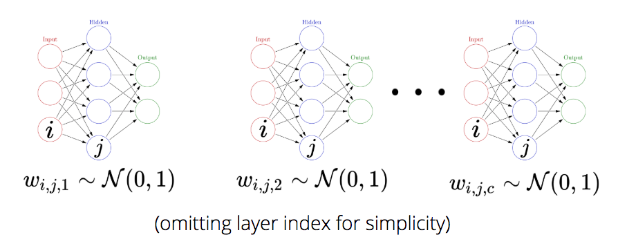
We use NUTS sampling here because the hierarchical model further below has a more complex posterior (see Why hierarchical models are awesome, tricky, and Bayesian for an explanation) and I wanted the results to be comparable. All simulations in here work with ADVI as well but the results don’t look quite as strong.
Ys_pred_train = []
Ys_pred_test = []
grid_eval = []

grid = pm.floatX(np.mgrid[-3:3:100j,-3:3:100j])
grid_2d = grid.reshape(2, -1).T
dummy_out = np.ones(grid.shape[1], dtype=np.int8)

for X_train, Y_train, X_test, Y_test in zip(Xs_train, Ys_train, Xs_test, Ys_test):
    pred_train, pred_test, ppc_grid, trace_flat = \
        fit_and_eval_bnn(X_train, X_test,
                         Y_train, Y_test,
                         grid_2d, dummy_out,
                         construct_flat_nn)
    Ys_pred_train.append(pred_train)
    Ys_pred_test.append(pred_test)
    grid_eval.append(ppc_grid)

Ys_pred_train = np.stack(Ys_pred_train)
Ys_pred_test = np.stack(Ys_pred_test)
ppc_grid_single = np.stack(grid_eval)
print ("Train accuracy = {:.2f}%".format(100*np.mean(Ys_pred_train == Ys_train)))Train accuracy = 86.78%print ("Test accuracy = {:.2f}%".format(100*np.mean(Ys_pred_test == Ys_test)))Test accuracy = 83.78%OK, that doesn’t seem so bad. Now let’s look at the decision surfaces – i.e. what the classifier thinks about each point in the data space.
fig, axs = plt.subplots(figsize=(15, 12), nrows=n_grps_sq, ncols=n_grps_sq, sharex=True, sharey=True)
axs = axs.flatten()
for i, (X, Y_pred, Y_true, ax) in enumerate(zip(Xs_train, Ys_pred_train, Ys_train, axs)):
    contour = ax.contourf(grid[0], grid[1], ppc_grid_single[i, ...].mean(axis=0).reshape(100, 100), cmap=cmap)
    ax.scatter(X[Y_true == 0, 0], X[Y_true == 0, 1], label='Class 0')
    ax.scatter(X[Y_true == 1, 0], X[Y_true == 1, 1], color='r', label='Class 1')
    sns.despine(); ax.legend()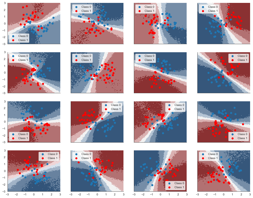
That doens’t look all that convincing. We know from the data generation process as well as from the previous blog post Bayesian Deep learning using the same data set that it give us a “Z”-shaped decision surface. So what happens is we don’t have enough data to properly estimate the non-linearity in every category.
Hierarchical Bayesian Neural Network
Can we do better? You bet!
It’s actually quite straight-forward to turn this into one big hierarchical model for all categories, rather than many individual ones. Let’s call the weight connecting neuron \(i\) in layer 1 to neuron \(j\) in layer 2 in category \(c\) \(w_{i, j, c}\) (I just omit the layer index for simplicity in notation). Rather than placing a fixed prior as we did above (i.e. $ w_{i, j, c} (0, 1^2)$), we will assume that each weight comes from an overarching group distribution: $ w_{i, j, c} (_{i, j}, ^2)$. The key is that we will estimate \(\mu_{i, j}\) and \(\sigma\) simultaneously from data.
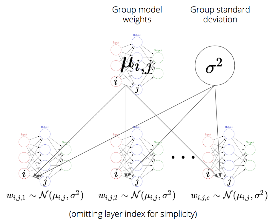
Why not allow for different \(\sigma_{i,j}^2\) per connection you might ask? Mainly just to make our life simpler and because it works well enough.
Note that we create a very rich model here. Every individual weight has its own hierarchical structure with a single group mean parameter and 16 per-category weights distributed around the group mean. While this creates a big amount of group distributions (as many as the flat NN had weights) there is no problem with this per-se, although it might be a bit unusual. One might argue that this model is quite complex and while that’s true, in terms of degrees-of-freedom, this model is simpler than the unpooled one above (more on this below).
As for the code, we stack weights along a 3rd dimenson to get separate weights for each group. That way, through the power of broadcasting, the linear algebra works out almost the same as before.
def construct_hierarchical_nn(Xs, Ys):
    n_hidden = 5
    n_grps = Xs.shape[0].eval()
    n_data = Xs.shape[2].eval()
    # Initialize random weights between each layer
    init_1 = floatX(np.random.randn(n_data, n_hidden))
    init_2 = floatX(np.random.randn(n_hidden, n_hidden))
    init_out = floatX(np.random.randn(n_hidden))

    with pm.Model() as neural_network:
        # Group mean distribution for input to hidden layer
        weights_in_1_grp = pm.Normal('w_in_1_grp', 0, sd=1,
                                 shape=(n_data, n_hidden),
                                 testval=init_1)
        # Group standard-deviation
        weights_in_1_grp_sd = pm.HalfNormal('w_in_1_grp_sd', sd=1.)

        # Group mean distribution for weights from 1st to 2nd layer
        weights_1_2_grp = pm.Normal('w_1_2_grp', 0, sd=1,
                                shape=(n_hidden, n_hidden),
                                testval=init_2)
        weights_1_2_grp_sd = pm.HalfNormal('w_1_2_grp_sd', sd=1.)

        # Group mean distribution from hidden layer to output
        weights_2_out_grp = pm.Normal('w_2_out_grp', 0, sd=1,
                                  shape=(n_hidden,),
                                  testval=init_out)
        weights_2_out_grp_sd = pm.HalfNormal('w_2_out_grp_sd', sd=1.)

        # Separate weights for each different model, just add a 3rd dimension
        # of weights
        weights_in_1_raw = pm.Normal('w_in_1',
                                     shape=(n_grps, n_data, n_hidden))
        # Non-centered specification of hierarchical model
        # see https://twiecki.github.io/blog/2017/02/08/bayesian-hierchical-non-centered/
        weights_in_1 = weights_in_1_raw * weights_in_1_grp_sd + weights_in_1_grp

        weights_1_2_raw = pm.Normal('w_1_2',
                                    shape=(n_grps, n_hidden, n_hidden))
        weights_1_2 = weights_1_2_raw * weights_1_2_grp_sd + weights_1_2_grp

        weights_2_out_raw = pm.Normal('w_2_out',
                                      shape=(n_grps, n_hidden))

        weights_2_out = weights_2_out_raw * weights_2_out_grp_sd + weights_2_out_grp

        # Build neural-network using tanh activation function
        # tt.batched_dot just calls .dot along an axis
        act_1 = pm.math.tanh(tt.batched_dot(Xs, weights_in_1))
        act_2 = pm.math.tanh(tt.batched_dot(act_1, weights_1_2))
        act_out = tt.batched_dot(act_2, weights_2_out)

        # Binary classification -> Bernoulli likelihood
        out = pm.Bernoulli('out', logit_p=act_out, observed=Ys)

    return neural_network
sample_kwargs = dict(init='advi+adapt_diag', tune=5000, chains=1,
nuts_kwargs={'target_accept': 0.9},
progressbar=False)
grid_3d = np.repeat(grid_2d[None, ...], n_grps, axis=0)
dummy_out_3d = np.ones((n_grps, grid.shape[1]), dtype=np.int8)
Ys_hierarchical_pred_train, Ys_hierarchical_pred_test, ppc_grid, trace_hier = \
fit_and_eval_bnn(
Xs_train, Xs_test,
Ys_train, Ys_test,
grid_3d, dummy_out_3d,
construct_hierarchical_nn,
sample_kwargs=sample_kwargs)Auto-assigning NUTS sampler...
Initializing NUTS using advi+adapt_diag...
Convergence achieved at 54100
Interrupted at 54,099 [27%]: Average Loss = 522.66
Sequential sampling (1 chains in 1 job)
NUTS: [w_2_out, w_1_2, w_in_1, w_2_out_grp_sd, w_2_out_grp, w_1_2_grp_sd, w_1_2_grp, w_in_1_grp_sd, w_in_1_grp]
Only one chain was sampled, this makes it impossible to run some convergence checksprint('Train accuracy = {:.2f}%'.format(100*np.mean(Ys_hierarchical_pred_train == Ys_train)))Train accuracy = 91.11%print('Test accuracy = {:.2f}%'.format(100*np.mean(Ys_hierarchical_pred_test == Ys_test)))Test accuracy = 89.78%Great – we get higher train and test accuracy. Let’s look at what the classifier has learned for each category.
fig, axs = plt.subplots(figsize=(15, 12), nrows=n_grps_sq, ncols=n_grps_sq, sharex=True, sharey=True)
axs = axs.flatten()
for i, (X, Y_pred, Y_true, ax) in enumerate(zip(Xs_train, Ys_hierarchical_pred_train, Ys_train, axs)):
    contour = ax.contourf(grid[0], grid[1], ppc_grid[:, i, :].mean(axis=0).reshape(100, 100), cmap=cmap)
    ax.scatter(X[Y_true == 0, 0], X[Y_true == 0, 1], label='Class 0')
    ax.scatter(X[Y_true == 1, 0], X[Y_true == 1, 1], color='r', label='Class 1')
    sns.despine(); ax.legend()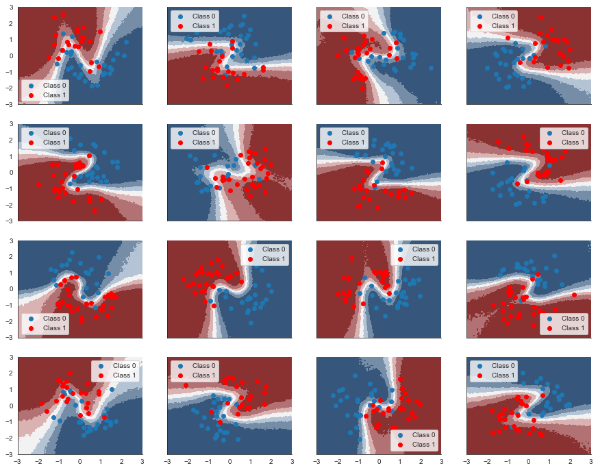
Awesome! By (partially) pooling the data for each individual category we actually manage to retrieve the non-linearity. This is the strength of hierarchical models: we model the similarities of individual categories and their differences, sharing statistical power to the degree it’s useful.
Of course, as we are in a Bayesian framework we also get the uncertainty estimate in our predictions:
fig, axs = plt.subplots(figsize=(15, 12), nrows=n_grps_sq, ncols=n_grps_sq, sharex=True, sharey=True)
axs = axs.flatten()
for i, (X, Y_pred, Y_true, ax) in enumerate(zip(Xs_train, Ys_hierarchical_pred_train, Ys_train, axs)):
    contour = ax.contourf(grid[0], grid[1], ppc_grid[:, i, :].std(axis=0).reshape(100, 100),
                          cmap=cmap_uncertainty)
    ax.scatter(X[Y_true == 0, 0], X[Y_true == 0, 1], label='Class 0')
    ax.scatter(X[Y_true == 1, 0], X[Y_true == 1, 1], color='r', label='Class 1')
    sns.despine(); ax.legend()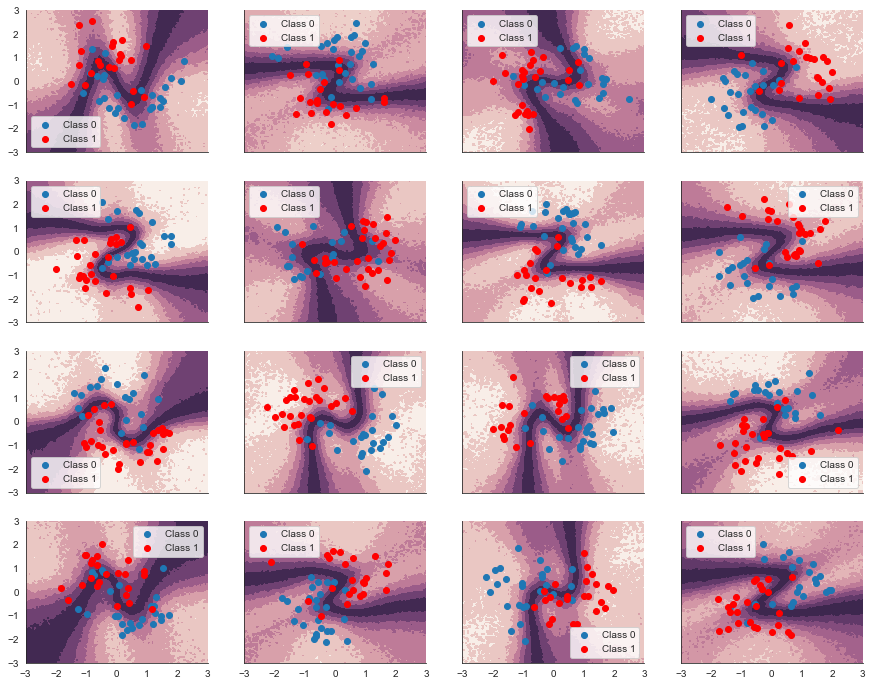
Further analysis
There are a couple of things we might ask at this point. For example, how much does each layer specialize its weight per category. To answer this we can look at the group standard-deviation which informs us how much each weight is allowed to deviate from its group mean.
pm.traceplot(trace_hier, varnames=['w_in_1_grp_sd', 'w_1_2_grp_sd', 'w_2_out_grp_sd']);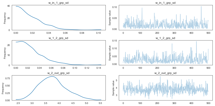
Interestingly, it seems that the specialization of the individual category sub-models is happening at the last layer where weights change most strongly from their group mean (as group variance is highest). I had assumed that this would happen at the first layer, based on what I found in my earlier blog post Random-Walk Bayesian Deep Networks: Dealing with Non-Stationary Data where the first layer acted as a rotation-layer.
Another interesting property of hierarchical models reveals itself here. As the group standard deviation is small for the weights in layers 1 and 2, it means these weights will be close to their group mean, reducing the effective number of parameters (degrees of freedom) of this model. This is different from the separate models where no similarities could be exploited to reduce the effective number of parameters. So from this perspective, the hierarchical model is simpler than the sum of the separate ones above.
Finally, I wondered what the group-model actually learned. To get at that, we can use the trace of \(\mu_{i,j}\) from the hierarchical model and pass it to the non-hierarchical model as if we trained these weights directly on a single data set.
trace_flat._straces[0].samples['w_in_1'] = trace_hier['w_in_1_grp']
trace_flat._straces[0].samples['w_1_2'] = trace_hier['w_1_2_grp']
trace_flat._straces[0].samples['w_2'] = trace_hier['w_2_out_grp']

ann_input = theano.shared(X_train)
ann_output = theano.shared(Y_train)
neural_network = construct_flat_nn(ann_input, ann_output)

with neural_network:
    # Evaluate classifier over grid
    ann_input.set_value(grid_2d)
    ann_output.set_value(dummy_out)
    ppc_grid_hier2 = pm.sample_ppc(trace_flat, samples=500,
                                   progressbar=False)['out']
contour = plt.contourf(grid[0], grid[1], ppc_grid_hier2.mean(axis=0).reshape(100, 100), cmap=cmap)
plt.xlabel('X1'); plt.ylabel('X2'); plt.title('Decision surface of the group weights');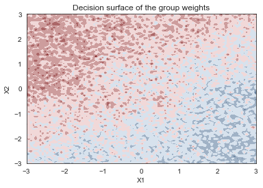
It seems like the group model is representing the Z-shape in a fairly noisy way, which makes sense because the decision surface for every sub-model looks quite different.
Correlations between weights
Usually we estimate NNs with MLE and BNNs with mean-field variational inference (like ADVI) which both ignore correlations between weights. As we used NUTS here, I was curious if there are meaningful correlations. Here, we look at the correlations in the first layer of the group distribution.
sns.clustermap(np.corrcoef(trace_hier[layer_names[0]].reshape((trace_hier[layer_names[0]].shape[0], -1)).T),
               vmin=-1, center=0, vmax=1)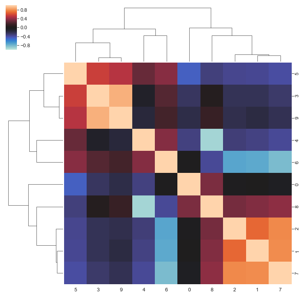
It indeed seems like point or mean-field estimates miss a lot of higher-order structure.
Informative priors for Bayesian Neural Networks
Informative priors are a powerful concept in Bayesian modeling. Any expert information you encode in your priors can greatly increase your inference.
The same should hold true for BNNs but it raises the question how we can define informative priors over weights which exist in this abstract space that is very difficult to reason about (understanding the learned representations of neural networks is an active research topic).
While I don’t know how to answer that generally, we can nonetheless explore this question with the techniques we developed this far. The group distributions from our hierarchical model are providing structured regularization for the subnetworks. But there is no reason we can’t use the group distributions only in a hierarchical network. We can just use the inferred group structure and reapply it in the form of informative priors to individual, flat networks.
For this, we must first estimate the group distribution as it looks to the subnetworks. The easiest approach is to draw sample \(l\) from the group posterior distributions (\(\mu_l\) and \(\sigma_l\)) and, using this sample, draw realizations \(x\) from the resulting distribution: \(x \sim \mathcal{N}(\mu_l, \sigma_l^2)\). This is essentially sampling from the group posterior predictive distribution.
from collections import defaultdict
samples_tmp = defaultdict(list)
samples = {}

for layer_name in layer_names:
    for mu, sd in zip(trace_hier.get_values(layer_name, chains=0),
                      trace_hier.get_values(layer_name+'_sd', chains=0)):
        for _ in range(20): # not sure why the `size` kwarg doesn't work
            samples_tmp[layer_name].append(stats.norm(mu, sd).rvs())
    samples[layer_name] = np.asarray(samples_tmp[layer_name])
While there is no guarantee that this distribution is normal (technically it is a mixture of normals so could look much more like a Student-T), this is a good enough approximation in this case. As the correlation structure of the group distributions seem to play a key role as we’ve seen above, we use MvNormal priors.
Note that this code just creates a single, non-hierarchical BNN.
def construct_flat_prior_nn(ann_input, ann_output, prior_1_mu=None, prior_1_cov=None,
                            prior_2_mu=None, prior_2_cov=None, prior_out_mu=None, prior_out_cov=None):
    n_hidden = 5

    with pm.Model() as neural_network:
        # In order to model the correlation structure between the 2D weights,
        # we flatten them first. Now here we have to reshape to give them their
        # original 2D shape.
        weights_in_1 = (pm.MvNormal('w_in_1', prior_1_mu.flatten(),
                                   cov=prior_1_cov,
                                   shape=prior_1_cov.shape[0])
                        .reshape((X.shape[1], n_hidden)))

        # Weights from 1st to 2nd layer
        weights_1_2 = (pm.MvNormal('w_1_2', prior_2_mu.flatten(),
                                  cov=prior_2_cov,
                                  shape=prior_2_cov.shape[0])
                       .reshape((n_hidden, n_hidden)))

        # Weights from hidden layer to output
        weights_2_out = (pm.MvNormal('w_2_out', prior_out_mu.flatten(),
                                    cov=prior_out_cov,
                                    shape=prior_out_cov.shape[0])
                         .reshape((n_hidden,)))

        # Build neural-network using tanh activation function
        act_1 = pm.math.tanh(pm.math.dot(ann_input,
                                         weights_in_1))
        act_2 = pm.math.tanh(pm.math.dot(act_1,
                                         weights_1_2))
        act_out = pm.math.dot(act_2, weights_2_out)

        # Binary classification -> Bernoulli likelihood
        out = pm.Bernoulli('out',
                           logit_p=act_out,
                           observed=ann_output)
    return neural_network
Again, we just loop over the categories in our data set and create a separate BNN for each one. This is identical to our first attempt above, however, now we are setting the prior estimated from our group posterior of our hierarchical model in our second approach.
Ys_pred_train = []
Ys_pred_test = []
grid_eval = []

for X_train, Y_train, X_test, Y_test in zip(Xs_train, Ys_train, Xs_test, Ys_test):
    n_samples = samples['w_in_1_grp'].shape[0]

    # Construct informative priors from previous hierarchical posterior
    bnn_kwargs = \
    dict(prior_1_mu=samples['w_in_1_grp'].mean(axis=0),
         prior_1_cov=np.cov(samples['w_in_1_grp'].reshape((n_samples, -1)).T),
         prior_2_mu=samples['w_1_2_grp'].mean(axis=0),
         prior_2_cov=np.cov(samples['w_1_2_grp'].reshape((n_samples, -1)).T),
         prior_out_mu=samples['w_2_out_grp'].mean(axis=0),
         prior_out_cov=np.cov(samples['w_2_out_grp'].reshape((n_samples, -1)).T))

    pred_train, pred_test, ppc_grid, _ = \
        fit_and_eval_bnn(X_train, X_test,
                         Y_train, Y_test,
                         grid_2d, dummy_out,
                         construct_flat_prior_nn,
                         bnn_kwargs=bnn_kwargs)

    Ys_pred_train.append(pred_train)
    Ys_pred_test.append(pred_test)
    grid_eval.append(ppc_grid)

Ys_info_pred_train = np.asarray(Ys_pred_train)
Ys_info_pred_test = np.asarray(Ys_pred_test)
grid_eval = np.asarray(grid_eval)
Drum roll
fig, axs = plt.subplots(figsize=(15, 12), nrows=n_grps_sq, ncols=n_grps_sq, sharex=True, sharey=True)
axs = axs.flatten()
for i, (X, Y_pred, Y_true, ax) in enumerate(zip(Xs_train, Ys_pred_train, Ys_train, axs)):
    contour = ax.contourf(grid[0], grid[1], grid_eval[i, ...].mean(axis=0).reshape(100, 100), cmap=cmap)
    ax.scatter(X[Y_true == 0, 0], X[Y_true == 0, 1], label='Class 0')
    ax.scatter(X[Y_true == 1, 0], X[Y_true == 1, 1], color='r', label='Class 1')
    sns.despine(); ax.legend()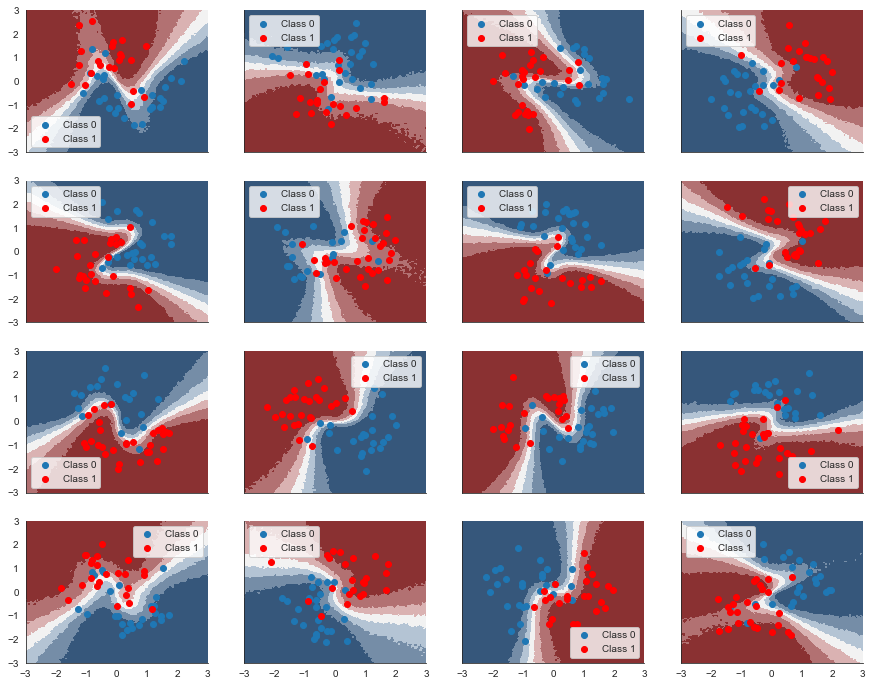
print('Train accuracy = {:.2f}%'.format(100*np.mean(Ys_info_pred_train == Ys_train)))Train accuracy = 91.56%print('Test accuracy = {:.2f}%'.format(100*np.mean(Ys_info_pred_test == Ys_test)))Test accuracy = 87.11%Holy mackerel, it actually worked!
As demonstrated, informed priors can help NNs a lot. But what if we don’t have hierarchical structure or it would be too expensive to estimate? We could attempt to construct priors by deriving them from pre-trained models. For example, if I wanted to train an object recognition model to my own custom categories, I could start with a model like ResNet trained on the CIFAR data set, derive priors from the weights, and then train a new model on my custom data set which could then get by with fewer images than if we trained from scratch.
Summary
In this blog post I showed how we can borrow ideas from Bayesian statistics (hierarchical modeling and informative priors) and apply them to deep learning to boost accuracy when our data set is nested and we may not have a huge amount of data.
If you want to play around with this notebook yourself, download it here.
Further reading
- Uncertainty in Multitask Transfer Learning: Great paper also using a hierarchical BNN but with more sophisticated inference and better benchmarks.
- Overcoming catastrophic forgetting in neural networks: Paper by DeepMind solving the same problem but with a different approach: they freeze certain weights when training on subsequent tasks.
Acknowledgements
If you enjoyed this blog post, please consider supporting me on Patreon.
Thanks to Adrian Seyboldt and Chris Chatham for useful discussions and feedback. Thanks also to my patrons, particularily Jonathan Ng and Vladislavs Dovgalecs.